PythonでFXのヒストリカルデータを元にボリンジャーバンドを描写する

FXヒストリカルデータを元にボリンジャーバンドを描写してみます。

前回の「FXのヒストリカルデータを元にPythonのpandasとmatplotlibを使用して移動平均線を描写する」で
移動平均線を描写していますので、ボリンジャーバンドの描写は簡単でした。

ボリンジャーバンドは、移動平均線を中心に上下に
+1σ（シグマ）、+2σ、-1σ、-2σ
の4本の線（移動平均線を含めると5本）の線を描写したものです。

移動平均線と同じくPandasのSeriesを使用します。
Pandasには、ボリンジャーバンドを描写するために必要な
σの値を算出する関数が用意されていますので、これを使用します。

ではさっそくプログラムソースです。

# -*- coding: utf-8 -*-
"""
Created on Tue Jan 10 16:44:16 2017

@author: ichizo
"""
import datetime
import sqlite3
import pandas as pd

import matplotlib.pyplot as plt
from matplotlib.finance import candlestick_ohlc

DB = 'usd_jpy_prices.db'
FROMDATE = '20161201000000'
TODATE = '20161201010000'
DTYPE = '1min'

def get_datas():
    conn = sqlite3.connect(DB)
    sql = "SELECT datetime, open, high, low, close FROM onemin WHERE datetime >= '%s' AND datetime <= '%s';" % (FROMDATE, TODATE)
    datas = pd.io.sql.read_sql_query(sql, conn)
    conn.close()

    return datas

def convert_datas(datas):
    datas['open'] = datas['open'].astype(float)
    datas['high'] = datas['high'].astype(float)
    datas['low'] = datas['low'].astype(float)
    datas['close'] = datas['close'].astype(float)

    if DTYPE == '1min':
        tmp = datas['datetime'].values.astype('datetime64[D]')
        datas['datetime'] = tmp.astype(float)
        return datas

    quotes_arr = []
    tmp_open_price = 0
    tmp_high_price = []
    tmp_low_price = []
    tmp_close_price = 0
    count = 0

    for loop, cDate in enumerate(datas['datetime']):
        isNext = False
        cDatetime = datetime.datetime.strptime(cDate, "%Y%m%d%H%M%S")

        if DTYPE == '5min' and cDatetime.minute % 5 == 0:
            isNext = True
        if DTYPE == '10min' and cDatetime.minute % 10 == 0:
            isNext = True
        if DTYPE == '30min' and cDatetime.minute % 30 == 0:
            isNext = True
        if DTYPE == '1hour' and cDatetime.minute == 0:
            isNext = True
        if DTYPE == '1day' and cDatetime.hour == 0:
            isNext = True
        
        if tmp_open_price == 0:
            tmp_open_price = datas['open'][loop]

        if isNext == True and loop != 0:
            data = []
            data.append(cDate)
            data.append(tmp_open_price)
            data.append(max(tmp_high_price))
            data.append(min(tmp_low_price))
            data.append(tmp_close_price)
            
            pddata = pd.DataFrame([data])
            pddata.columns = ["datetime", "open", "high", "low", "close"]
            pddata.index = [count]
            quotes_arr.append(pddata)

            tmp_open_price = datas['open'][loop]
            tmp_high_price = []
            tmp_low_price = []
            count += 1

        tmp_high_price.append(datas['high'][loop])
        tmp_low_price.append(datas['low'][loop])
        tmp_close_price = datas['close'][loop]

    for idx, value in enumerate(quotes_arr):
        if idx == 0:
            quotes = quotes_arr[idx]
        else:
            quotes = pd.concat([quotes, value],axis=0)

    quotes['datetime'] = quotes['datetime'].astype(float)
    quotes['open'] = quotes['open'].astype(float)
    quotes['high'] = quotes['high'].astype(float)
    quotes['low'] = quotes['low'].astype(float)
    quotes['close'] = quotes['close'].astype(float)

    return quotes

if __name__ == '__main__':
    datas = get_datas()
    datas = convert_datas(datas)

    plt.grid()
    ax = plt.subplot()
    candlestick_ohlc(ax, datas.values, width=200.0, colorup='#77d879', colordown='#db3f3f')
    
    #移動平均線
    s = pd.Series(datas['close'])
    sma25 = s.rolling(window=25).mean()
    #sma5 = s.rolling(window=5).mean()
    #plt.plot(datas['datetime'], sma5)
    deviation = 2
    sigma = s.rolling(window=25).std(ddof=0) #σの計算
    upper_siguma = sma25 + sigma
    upper2_siguma = sma25 + sigma * deviation
    lower_siguma = sma25 - sigma
    lower2_siguma = sma25 - sigma * deviation

    plt.plot(datas['datetime'], sma25)
    plt.plot(datas['datetime'], upper_siguma)
    plt.plot(datas['datetime'], upper2_siguma)
    plt.plot(datas['datetime'], lower_siguma)
    plt.plot(datas['datetime'], lower2_siguma)

    plt.xlabel('Date')
    plt.ylabel('Price')
    plt.title('USD-JPY')
    plt.show()

今回追加したのは以下の部分です。

    deviation = 2
    sigma = s.rolling(window=25).std(ddof=0) #σの計算
    upper_siguma = sma25 + sigma
    upper2_siguma = sma25 + sigma * deviation
    lower_siguma = sma25 - sigma
    lower2_siguma = sma25 - sigma * deviation

    plt.plot(datas['datetime'], sma25)
    plt.plot(datas['datetime'], upper_siguma)
    plt.plot(datas['datetime'], upper2_siguma)
    plt.plot(datas['datetime'], lower_siguma)
    plt.plot(datas['datetime'], lower2_siguma)

σの値は、

sigma = s.rolling(window=25).std(ddof=0)

で計算できますので、この値を移動平均線の値にプラス（もしくはマイナス）するだけです。

出力した結果は以下になります。

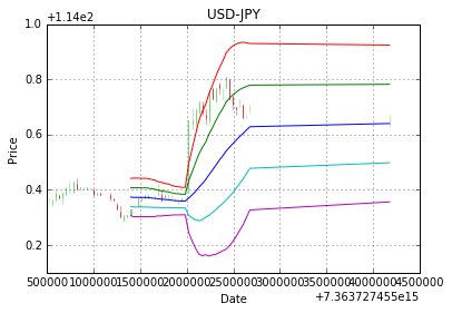
それっぽいグラフになりました。